Phased Array Microphone

A 192-channel phased array microphone, with FPGA data acquisition and beamforming/visualization on the GPU. Phased arrays allow for applications not possible with traditional directional microphones, as the directionality can be changed instantly, after the recording is made, or even be focused at hundreds of thousands of points simultaneously in real time.

All designs are open source:

• Host software
• FPGA gateware
• PCB layout and schematics, mechanical components

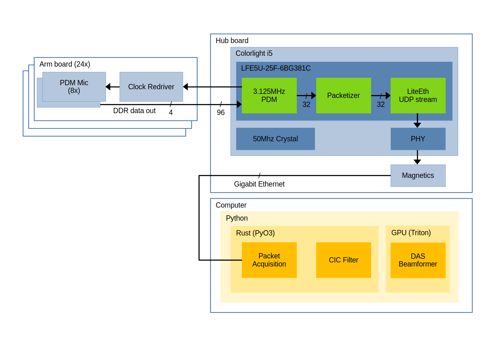
Block diagram

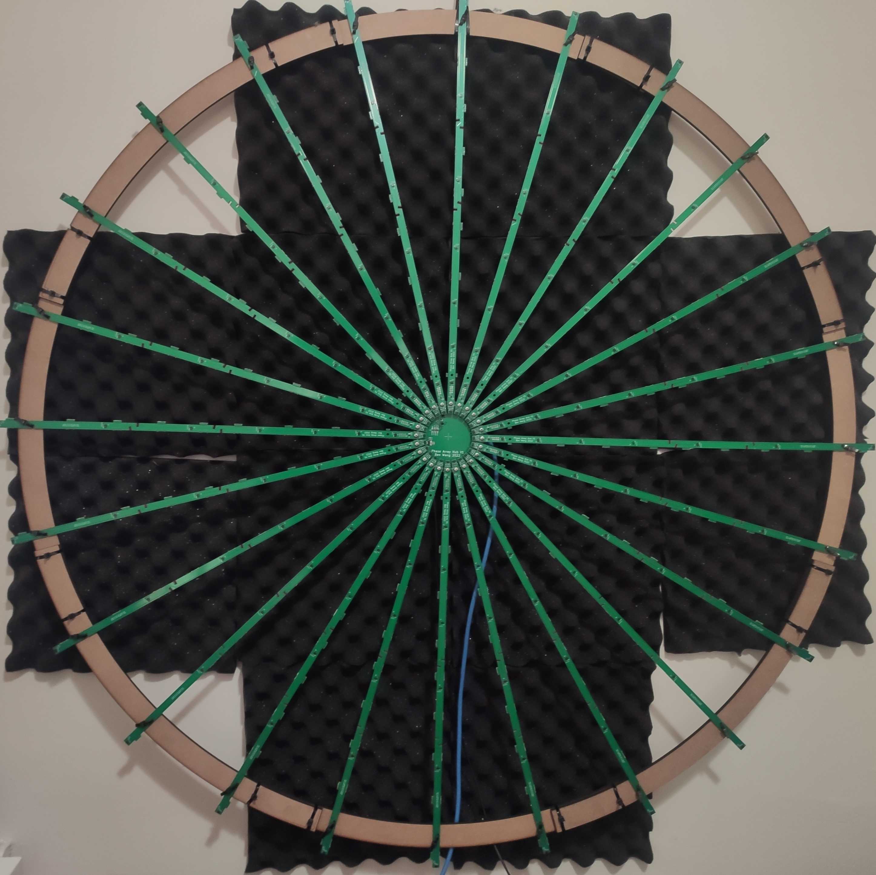
Glamor shot

Hardware

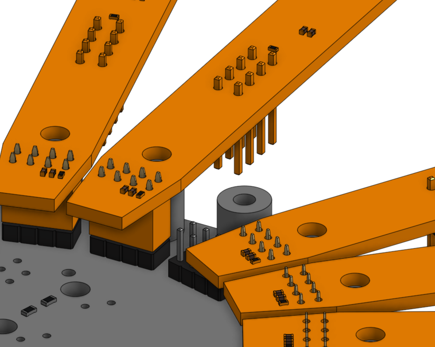
To create a phased array microphone, a large number of microphones needs to be placed in an arrangement with a wide distribution of spacing. For a linear array, exponential spacing between microphones is found to be optimal for broadband signals. To create a 2d array, these symmetrical linear arrays (“arms”) are be placed radially, which allows the central (“hub”) board to be compact. The total cost for the array is approximately $700.

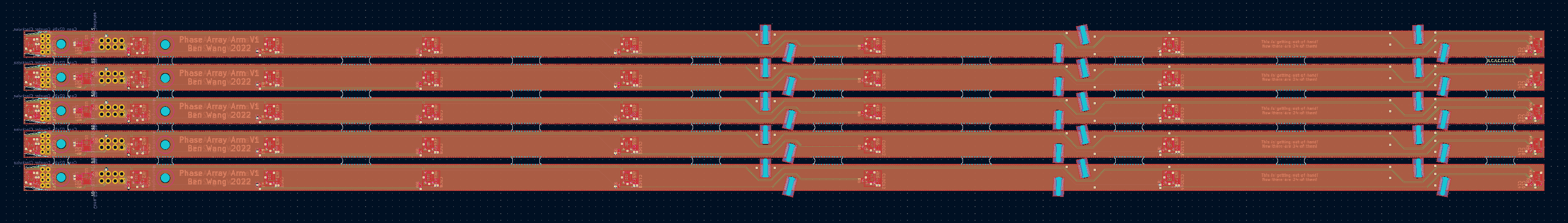
Arms

The length of each arm is dictated by the limits of PCB manufacturing and assembly. These boards were made at JLCPCB, where the maximum length for manufacturing and assembly of 4 layer PCBs was 570mm.

The microphones chosen were the cheapest digital output MEMS microphone (because there are a lot of them!), which were about $0.5. At this bottom of the barrel price range, there is little differentiation in the performance characteristics between different microphones. Most have decent performance up to 10khz and unspecified matching of phase delay and volume.

These microphones output data using pulse density modulation (PDM), which provides a one bit output at a frequency significantly higher than the audible range (up to 4 MHz), with the high sampling rate compensating for quantization noise. These microphones also support latching the data either on the rising or falling edge of the clock (DDR), which allows two microphones to be multiplexed on a single wire, reducing the amount of connections required.

Each arm contains 8 microphones sharing 4 output lines, as well as an output buffer on the clock input line. This ensures the rise times are reasonable, even with hundreds of microphones sharing the same clock signal.

For some reason (likely the low rigidity of the panel and some suboptimal solder paste stencil patterns combined with the LGA microphone footprints), the yields on the arm PCBs are not very good, with only 50% of them working out of the box. The most common fault was the clock line being shorted to either 3V3 or ground, which unfortunately requires trial and error of removing microphones from the PCB until the short is resolved. Next time some series resistors on the clock line would speed this process up a lot, and improving the panelization and paste stencil would likely improve yields so extensive rework isn’t required.

Even with rework, there are still some microphones which produce bogus data. These are just masked out in the code, as there are enough working ones to make up for it (and it’s too much work to remove a bunch of arms to do more rework…)

Hub

An FPGA is used to collect all the data, due to the large number of low latency IOs available combined with the ability to communicate using high speed interfaces (e.g. Gigabit Ethernet). Specifically, the Colorlight i5 card is used, as it has enough IOs, is cheap and readily available, and has two integrated ethernet PHYs (only one is used for this project). The card is originally designed as an ethernet interface for LED panels, but has been fully reverse engineered. About 100 GPIOs are broken out over the DDR2 connector, which is much easier to fan out than the BGA of the original FPGA.

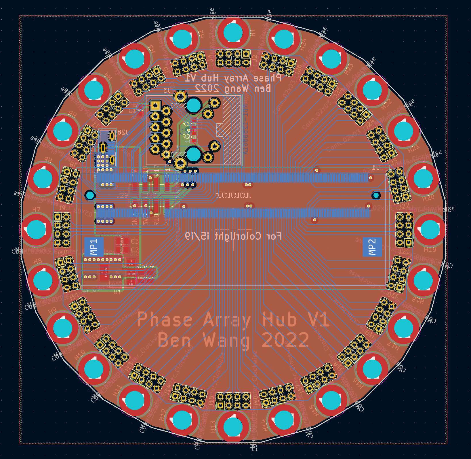
Other than the FPGA, the hub contains some simple power management circuitry, and connectors for the arm boards as well as an Ethernet connector with integrated magnetics.

Mechanical Design

The arms are attached with M3 screws to the hub using PCB mounted standoffs/nuts , which conveniently can be assembled with SMD processes. The connections from each arm to the hub is made with 8 pin, 2mm pitch connectors.

The original mechanical design consists of slots on the arm PCBs which interlock with circumferential structural PCBs, however the low torsional rigidity of the arms means the whole structure deformed too easily.

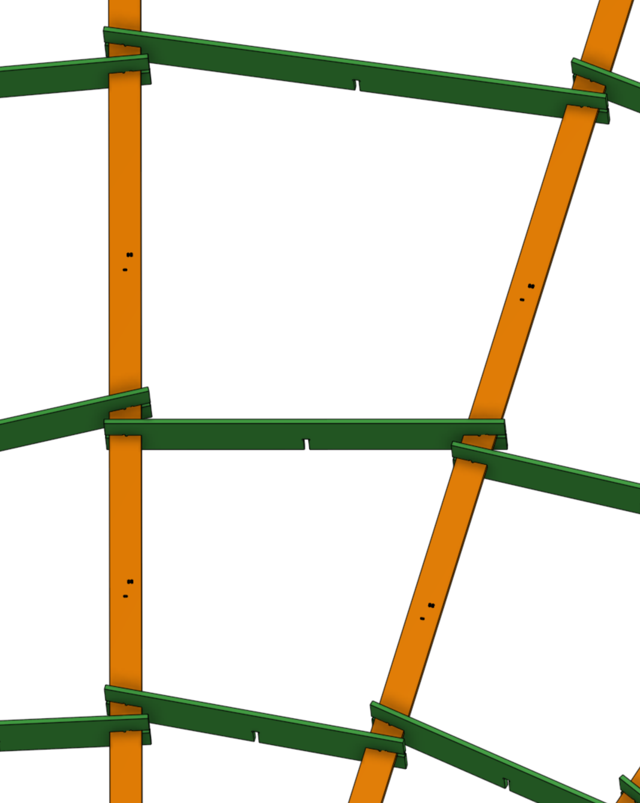
The final mechanical design consists of pieces of laser cut 1/4th inch MDF around the outer edge of the array, with each arm attached to the MDF with some zip ties.

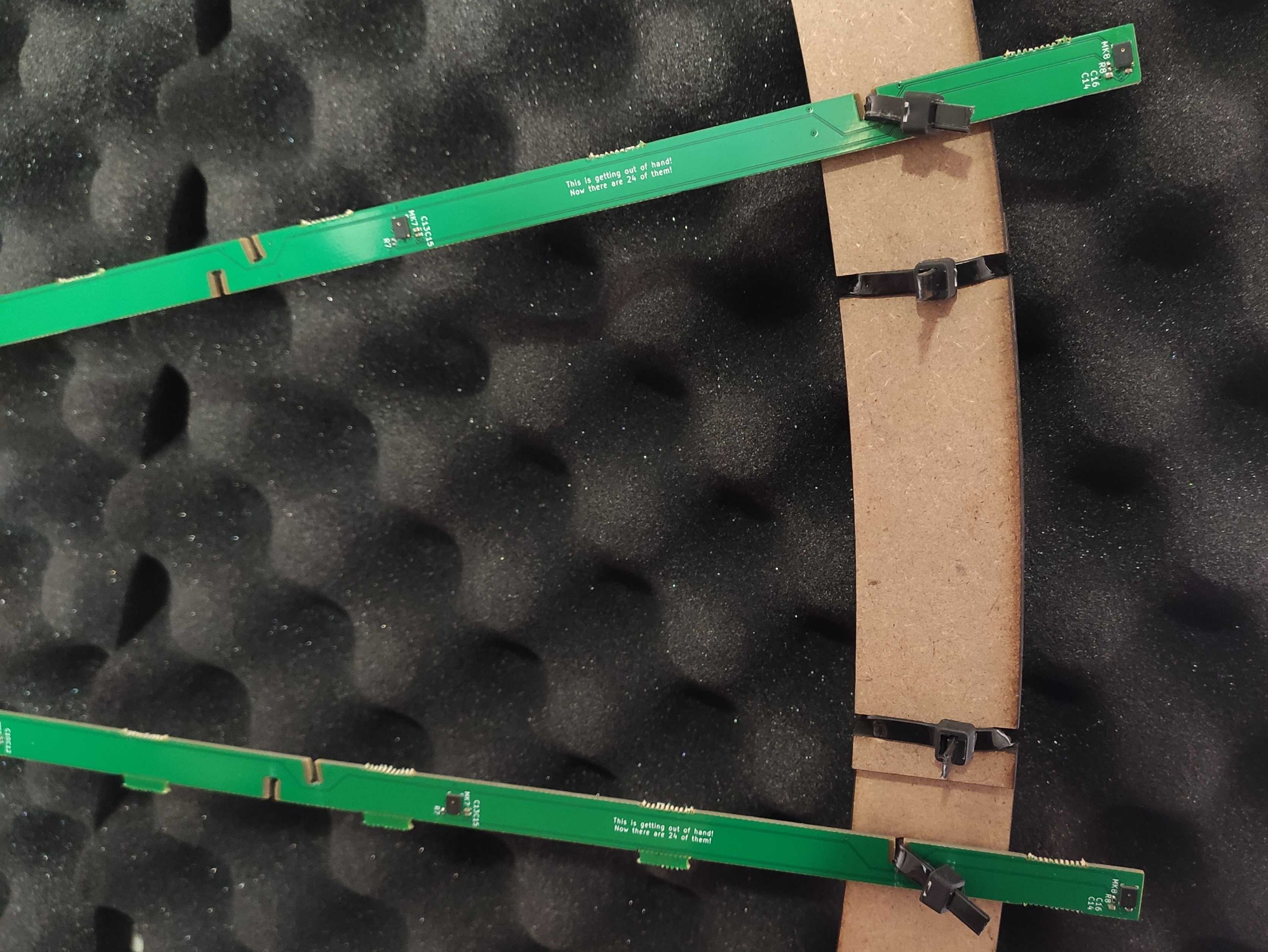
As the microphone array is mounted on the wall (which is very susceptible to reflections), a layer of acoustic foam is used to attenuate the reflections to make calibration easier.

Gateware

The main objective for the gateware is to reliably transmit the raw acquired data losslessly to the computer for further processing, while keeping it as simple as possible. Performing decimation and filtering on the FPGA would reduce the data rate, but sending the raw PDM data is achievable with Gigabit Ethernet. This reduces the complexity of the FPGA code and allowing faster iteration. Compiling is much faster than place and route, and it’s much easier to use a debugger in code than in gateware!

There are three major components to the gateware, a module for interfacing with the PDM interfaces, a module for creating fixed size packets from those readings, and a UDP streamer to write the packets to the Ethernet interface.

PDM Interface

The PDM input module is a relatively simple piece of logic, which divides the 50 MHz system clock by a factor of 16 to output a 3.125MHz PDM clock, latches all 96 of the input pins after each clock edge, and then shifts out 32 bits of the data on each clock cycle. Each chunk of 192 bits is has a header added which is a 32 bit incrementing integer.

The PDM interface receives data at a rate of 3.125Mhz * 96 (input pins) * 2 (DDR), which is 600Mbps. With the header, the data rate output from this module is 700Mbps, or approximately 40% utilization of the 32 bit output data path.

Packetizer

The packetizer is essentially a FIFO buffer with a special interface on the input. A standard FIFO marks the output as available whenever there is at least one item in the queue, but this would lead to smaller packets than requested as the ethernet interface operates faster than the PDM output (leading to buffer underruns). Thus, the packetizer waits until there is at least a full packet worth of data in the queue before starting a packet, which ensures constant sized packets.

48 PDM output blocks at 224 bits (192 bits of data with a 32 bit header) are placed into each packet, which totals 1344 bytes of data per packet, plus a 20 byte IPv4 header and an 8 byte UDP header, at a rate of approximately 65k pps.

This leads to a wire rate of 715 Mbps, or about 70% utilization of Gigabit Ethernet.

UDP Streamer

The LiteEth project made this module very easy, as it abstracts out the lower level complexities of UDP and IP encapsulation, ARP tables and the like, and provides a convenient interface for simply hooking up a FIFO to a UDP stream. Occasionally there is some latency, but there is enough slack in the bus and buffer in the packetizer FIFO to absorb any hiccups.

Utilization and Timing

The FPGA on the Colorlight i5 is a LFE5U-25F-6BG381C, which has 25k LUTs. The design is placed and routed with the open source Project Trellis toolchain. By keeping the gateware very simple, the utilization on the device is quite low, and there is lots of room for additional functionality.

Info: Device utilisation:
Info:                 DP16KD:    16/   56    28%
Info:                EHXPLLL:     1/    2    50%
Info:             TRELLIS_FF:  1950/24288     8%
Info:           TRELLIS_COMB:  3701/24288    15%
Info:           TRELLIS_RAMW:    49/ 3036     1%

Info: Max frequency for clock                   '$glbnet$crg_clkout': 73.17 MHz (PASS at 50.00 MHz)
Warning: Max frequency for clock '$glbnet$eth_clocks1_rx$TRELLIS_IO_IN': 124.07 MHz (FAIL at 125.00 MHz)

(Timing violations on eth rx clock is due to false positive from gray counter in liteeth)

Software

CIC Filter

Each microphone produces a 1 bit signal at 3.125Mhz, and needs to be reduced to a more reasonable sample rate and bit depth for further processing. This is done very efficiently with a CIC filter, which only requires a few arithmetic operations to process each sample. For understanding more about CIC filters, this series of blog posts from Tom Verbeure provides an excellent introduction. Following the nice graphs from there, I decided on a 4 stage, 16x decimation CIC filter which reduced the sample rate to a much reasonable 195kHz, at 32 bits.

To ingest the data at 3.125Mhz, the filter must be able to process each set of samples in 320ns. A naive implementation in Rust wasn’t fast enough on a single core, but an implementation with some less abstraction (and a hence some more autovectorization) got there, and is what was used at the end. I also experimented with a version using SIMD intrinsics which was much faster, but ended up running into alignment issues when using it in together with other code.

Even with close to a billion bits per second of data to process, a single CPU core can do quite a few operations on each individual bit!

test cic::bench_cic       ... bench: 574 ns/iter (+/- 79) = 41 MB/s
test cic::bench_fast_cic  ... bench: 181 ns/iter (+/- 24) = 132 MB/s
test cic::bench_simd_cic  ... bench:  36 ns/iter (+/- 0)  = 666 MB/s

Calibration

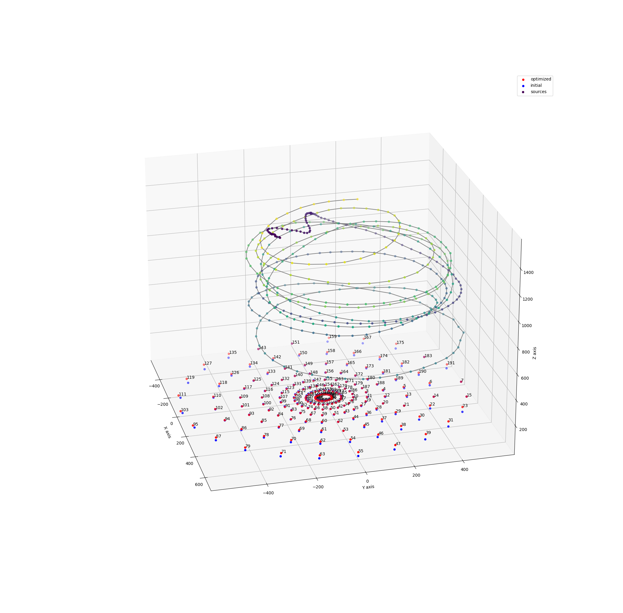
To perform array calibration, a speaker playing white noise is moved around the room in front of the array. An FFT based cross correlation is performed between all pairs of microphones to compute relative delays.

A cross correlation can be performed by computing the FFT of both signals (cached and computed once for each signal), and then computing the inverse FFT of the complex multiplication of the two. This is quite compute intensive, as there are over 18 thousand pairs! For the window sizes used of 16-64k, the FFTs are memory bound, and thus the IFFT and peak finding is fused to avoid writing the results to memory, which results in a 15x speedup. On a 7950X, this process runs in realtime.

Then the positions of the source at each timestep and the positions of each microphone is optimized using gradient descent (when you know PyTorch, all optimization problems look like gradient descent…). The loss function tries to minimize the difference between the measured correlations and the ideal correlations, while trying to minimize the deviation of the microphone positions from the initial positions as well as the jerk of the source trajectory.

As part of the calibration, the speed of sound is also a parameter which is optimized to obtain the best model of the system, which allows this whole procedure to act as a ridiculously overengineered thermometer.

After a few hundred iterations, it converges to a reasonable solution for both the source positions and the microphone positions, as well as constants such as the speed of sound. Fortunately this problem vectorizes well for GPU, and converges in a few seconds.

The final mean position error is on the order of 1mm, and is able to correct for large scale systematic distortions such as concavity from the lack of structural rigidity. The largest position error between the calibrated positions and the designed positions is on the order of 5mm, which is enough to introduce significant phase errors to high frequency sound if uncorrected, although perhaps not strictly necessary (10khz sound has a wavelength of ~3.4cm).

Beamforming

Beamforming is how the raw microphone inputs are processed to produce directional responses. The simplest method of beamforming is delay-and-sum (DAS), where each signal is delayed according to its distance from the source. This is the type of beamforming implemented for this process, with the beamforming happening in the frequency domain.

In the frequency domain, a delay can be implemented by the complex multiplication of the signal with a linear phase term proportional to the delay required, which also nicely handles delays which are not integer multiples of the sampling period.

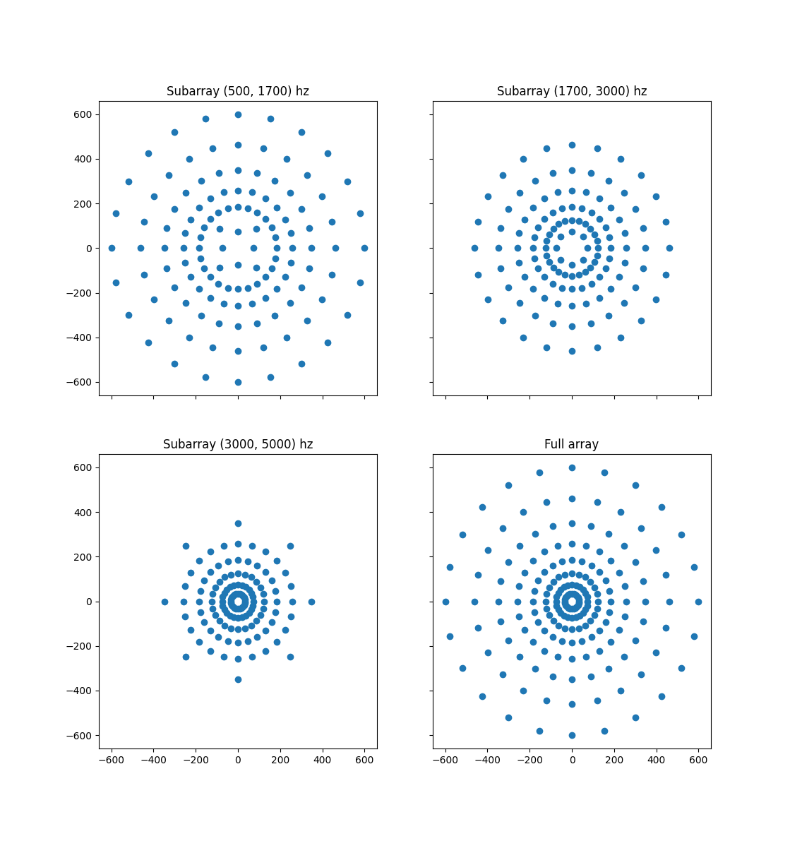
Multiple nested subarrays of the original array are used for different frequency ranges. This reduces the processing required for beamforming, as each frequency does not need to be beamformed with all the microphone. This also ensures that the beamforming gains of all the frequencies are matched.

Two different types of beamforming visualizations are implemented, a 3d near field beamformer and a 2d far field beamformer. When the audio source is far away, the wavefront is essentially a flat plane, and how far away the source is does not meaningfully change the signals at the array. On the other hand, if the source is close to the array, the wavefront will have a significant curvature which allows the 3d location of the source to be determined.

The beamformer is implemented as a Triton kernel, a Python DSL which compiles to run on Nvidia GPUs. When beamforming to hundreds of thousands of points, the massive parallelism provided by GPUs allows for results to be produced in real time. Some current limitations with the Triton language around support to indexing with shared memory arrays lead to slightly suboptimal performance, but writing CUDA C++ doesn’t seem very fun…

Near Field 3D Beamforming

Near field 3D beamforming is performed a 5cm voxel grid with size 64x64x64. An update rate of 12hz is achieved on a RTX 4090 with higher update rates limited by overhead of suboptimal CPU-GPU synchronization with the smaller work units. The voxel grid is then visualized using VisPy, a high performance data visualization library which uses OpenGL. Modern games have millions of polygons, so rendering a quarter million semi-transparent voxels at interactive framerates is no issue.

A quick demo of the voxel visualization below, note the reflection off the roof!

Far Field 2D Beamforming

Far field beamforming works similarly, but can be performed in higher resolution as there is no depth dimension required. A 512x512 pixel grid is used, and the same 12hz update rate achieved. (The far field beamforming uses an approximation of just putting the points far away instead of actually assuming planar wavefront due to laziness…)

A demo of the 2d visualization here, but it’s not very exciting due to the poor acoustic environment of my room around the array, with lots of reflections and multipath.

Directional Audio

The previous two beamforming implementations compute the energy of sound from each location, but never materializes the beamformed audio in memory. A time domain delay and sum beamformer is implemented to allow for directional audio recording. It takes a 3D coordinate relative from array center and outputs audio samples. An interesting aspect about this beamformer is that it is differentiable with regard to the location from the output. This means the location of the audio sources can be optimized based on some differentiable loss function (like neural network), which might allow for some interesting applications such as using a forced alignment model of a multi-party transcript to determine the physical location of each speaker.

A speaker playing some audio is placed in front of the array, with another speaker placed approximately 45 degrees away at the same distance from array center, playing white noise. The effectiveness of the beamforming can be demonstrated by comparing the raw audio from a single microphone with the output from the beamforming.

Raw audio from a single microphone:

Beamformed audio:

Recording

As the data from the microphone array is just UDP packets, it can be recorded with tools like tcpdump, and the packet capture file can be read to reinject the packets back into the listener. All the programs in the previous sections are designed to work at real time, but can also work on recorded data using this process.

The tradeoff with this recording implementation is that the output data rate is quite high (due to faithfully recording everything, even the quantization noise). At 87.5 MBps, a 1-hour recording would be 315 GB! A more optimized implementation would do some compression, and do the recording after the CIC filter at a lower sample rate.

Next Steps

I consider this project essentially complete, and don’t plan to work on it any further for the foreseeable future, but there are still lots of possible cool extensions if you’d like to build one!

• Using more advanced beamforming algorithms (DAMAS etc.)
• Better GUI to combine all existing functions (e.g. See where sound is coming from, and record audio from there)
• Combine differentiable beamforming and neural models (e.g. forced alignment example mentioned above)